
Descriptive Statistics
[!tldr] Summary 1st approach to statistics 101
[!quote] Quote .
This module is about statistics. First one need to define this concept. Indeed, the word statistics is both the collection of observed data and the set of methods used to gather, process, and analyse these data. For instance, recording the number crashs on a road constitutes a statistical dataset. Statistical methods are widely used in plenty of domain. This is just here to have the general principles.
Statistic or statistics?
In English, one can hear statistics and statistic. Statistic actually refers to a measure, a quantity, a datum obtained from a study ( mean, median for instance) from a data collection. Statisitcs refers to the field of collecting, analysing interpreting and communicating data. It is the science of interacting with data.
Definitions, vocabulary
- Population: Refers to any kind of set.
- Variable or feature: Refers to an application in set theory.
- Individual or Statistical Unit: Refers to an element in set theory.
- Subpopulation: Refers to a subset.
- Cardinality: Refers to the size or count. Set Theory Term | Statistical Term |
Definition
The frequency of a subpopulation \(E\) of \(\Omega\) is the ratio of the size of \(E\) and \(\Omega\):
\(f(E) = \frac{\text{Card}(E)}{\text{Card}(\Omega)} \in [0, 1]\)
Example
If we consider 200 records of games of Civilization VI, we obtain the following table:
| Type of civilisation | Count | Frequency |
|---|---|---|
| Scientific | 80 | 40% |
| Military | 60 | 30% |
| Cultural | 40 | 20% |
| Other | 20 | 10% |
| Total | 200 | 100% |
This frequency is often expressed as a percentage.
Statistics and probabilities
Probability theory plays a crucial role in statistics as it allows modeling random phenomena—experiments whose outcomes cannot be predicted with certainty. For instance, if a fair die is rolled 6000 times, we expect the number of times “6” appears to be around 1000. Probability theory formalises these intuitions, and statistics confront probabilistic models with observed reality to validate or invalidate them.
Variables / Features
In statistics, the population, generally denoted as \(\Omega\), is a set of unambiguously defined elements called individuals. The population is the reference universe in a statistical study.
Example 2: Tie Defender production line
Let’s study the Tie Defender produced in a series at a specific Imperial shipyard. We define the population \(\Omega\) as the set of all Tie Fighters produced at the Lothal factory during a year (1BBY).
Each individual in a population is described by a set of characteristics called variables or features.
Qualitative Variables express membership in a category.
- Example: For the Tie Defender, the feature “sabotaged by Rebels” is qualitative (Yes/No).
Quantitative (or Numerical) Variables are measured numerically.
- Examples: Engine power output, laser cannon recharge rate, hull integrity percentage are quantitative variables.
Example 3
The number of protocol errors observed in a C-Series protocol droid during a standard diplomatic reception is a discrete variable. You can count them: 0 errors, 1 error, 2 errors, etc.
Given a discrete variable \(X\), the set of values (or modalities) taken by \(X\) is the set: \(X(\Omega) = \{ x_{1}, x_{2}, \ldots, x_{n}, \ldots \} = \{ x_{i}, i \in \mathbb{N}^{*} \}\)
If we denote \(n_{i}\) as the number of occurrences of \(x_{i}\) in the entire population, and \(n = \text{Card}(\Omega)\) as the size of the population, then the corresponding frequency is: \(f_{i}= \frac{n_{i}}{n}\)
Example 4
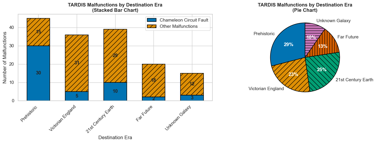
The following table shows the distribution of 155 recorded TARDIS malfunctions categorized by the destination time period the Doctor was attempting to reach.
| Destination Era \(x_i\) | Number of malfunctions \(n_{i}\) | Frequency \(f_{i}\) |
|---|---|---|
| Prehistoric | 45 | 29% |
| Victorian England | 36 | 23% |
| 21st century Earth | 36 | 25% |
| Far future | 20 | 13% |
| Unknown galaxy | 15 | 10% |
| Total | 155 | 100% |
We represent the counts (effectifs) or frequencies using appropriate diagrams:
- Bar Charts: The count or frequency corresponding to each value of the characteristic is represented by the length of a bar. Multiple data series can be represented on the same graph using stacker or grouped bar, as bellow.
- Pie Charts: Each value or class is represented by a sector of a disk whose angle (and thus area) is proportional to its frequency
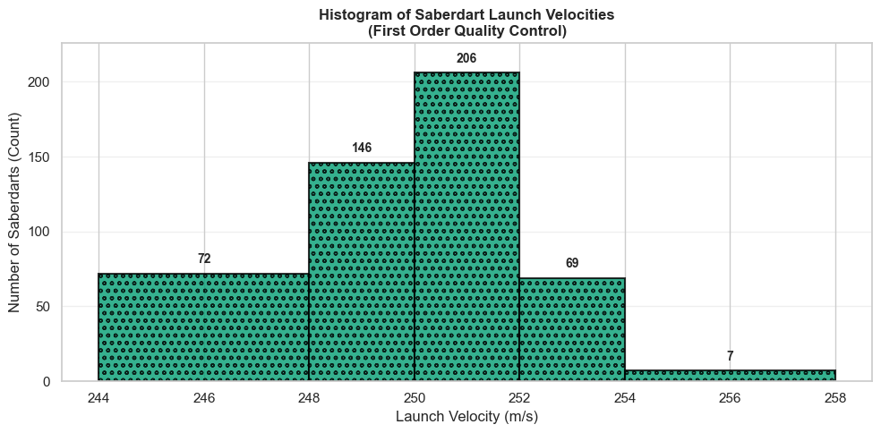
A characteristic is said to be continuous when the values it can take constitute an interval of \(\mathbb{R}\). In this case, it is common to divide the population into classes based on intervals of values taken by the characteristic. This process is sometimes called discretization of the variable.
Example 5
The time \(X\) it takes for a civilisation in Sid Meir’s Civilization VI to build a specific wonder is a continuous variable. It could be any value within a range, depending on production output.
In this case, we group the observed values into \(k\) classes with endpoints \(e_{0}, e_{1}, \ldots, e_{k}\) and we note for each class \([e_{i-1},e_{i}]\) the count \(n_{i}\), the frequency \(f_{i}\), as well as the cumulative frequencies:
\(F_{i}= \sum\limits_{j=1}î f_{j}\) We can then observe that \(F_{i}\) is the proportion of individuals for which \(X < e_{i}\).
Exemple 6
The First Order’s quality control division measures the launch velocity \(X\) of saberdarts (in meters per second) produced by a specific factory. The following table gives the distribution by class for a sample of 500 saberdarts.
| Velocity (\(ms^{-1}\)) | Count \(n_i\) | Frequency (%) | Cumulative Frequency (%) |
|---|---|---|---|
| \([244;248]\) | 72 | 14.4 | 14.4 |
| \([248;250]\) | 146 | 29.2 | 43.6 |
| \([250;252]\) | 206 | 41.2 | 84.8 |
| \([252;254]\) | 69 | 13.8 | 98.6 |
| \([254;258]\) | 7 | 1.4 | 100 |
| Total | 500 | 100 |
We can represent this data series with a histogram: each class is represented by a rectangle whose area is proportional to the count
These plots are generated using
import matplotlib.pyplot as plt
import numpy as np
import seaborn as sns

# Set colorblind-friendly style
sns.set_theme(style="whitegrid")
colorblind_palette = sns.color_palette("colorblind")

# Data from Example 4
categories = ['Prehistoric', 'Victorian England', '21st Century Earth', 'Far Future', 'Unknown Galaxy']
malfunctions = [45, 36, 39, 20, 15]
frequencies = [29, 23, 25, 13, 10] # in percent

# --- FIGURE 2: Stacked Bar Chart ---
# Let's imagine we break down malfunctions into two types: 'Chameleon Circuit' and 'Other'
chameleon_malfunctions = [30, 5, 10, 2, 3]
other_malfunctions = [m - c for m, c in zip(malfunctions, chameleon_malfunctions)]

fig, (ax1, ax2) = plt.subplots(1, 2, figsize=(14, 5))

# Bar Chart (Stacked) with patterns
bar_width = 0.6
x_pos = np.arange(len(categories))

# Create stacked bars with different patterns
bars1 = ax1.bar(x_pos, chameleon_malfunctions, bar_width,
                label='Chameleon Circuit Fault',
                color=colorblind_palette[0],
                edgecolor='black', linewidth=1.2)

bars2 = ax1.bar(x_pos, other_malfunctions, bar_width,
                bottom=chameleon_malfunctions,
                label='Other Malfunctions',
                color=colorblind_palette[1],
                hatch='//',  # Add pattern for distinction
                edgecolor='black', linewidth=1.2)

ax1.set_title('TARDIS Malfunctions by Destination Era\n(Stacked Bar Chart)', fontweight='bold')
ax1.set_ylabel('Number of Malfunctions')
ax1.set_xlabel('Destination Era')
ax1.set_xticks(x_pos)
ax1.set_xticklabels(categories, rotation=45, ha='right')
ax1.legend()

# Add value labels on bars
for bar in bars1:
    height = bar.get_height()
    if height > 0:
        ax1.text(bar.get_x() + bar.get_width()/2., bar.get_y() + height/2,
                f'{int(height)}', ha='center', va='center', fontweight='bold')

for bar in bars2:
    height = bar.get_height()
    if height > 0:
        ax1.text(bar.get_x() + bar.get_width()/2., bar.get_y() + height/2,
                f'{int(height)}', ha='center', va='center', fontweight='bold')

# --- FIGURE 3: Pie Chart with patterns and labels ---
# Pie Chart with explicit labels and patterns
wedges, texts, autotexts = ax2.pie(malfunctions,
                                   labels=categories,
                                   autopct='%1.0f%%',
                                   startangle=90,
                                   colors=colorblind_palette,
                                   wedgeprops={'edgecolor': 'black', 'linewidth': 1.2})

# Add patterns to pie chart wedges
patterns = ['', '//', '\\\\', '||', '--']
for wedge, pattern in zip(wedges, patterns):
    wedge.set_hatch(pattern)

ax2.set_title('TARDIS Malfunctions by Destination Era\n(Pie Chart)', fontweight='bold')

# Make percentage labels bold and white for better contrast
for autotext in autotexts:
    autotext.set_color('white')
    autotext.set_fontweight('bold')

plt.tight_layout()
plt.show()

# --- FIGURE 4: Histogram for Example 6 ---
# Data from Example 6
velocities = [244, 248, 250, 252, 254, 258] # Bin edges
counts = [72, 146, 206, 69, 7] # This is n_i. For a histogram, we use the counts directly.

# Calculate bin widths and centers for plotting
bin_widths = [velocities[i+1] - velocities[i] for i in range(len(velocities)-1)]
bin_centers = [(velocities[i] + velocities[i+1])/2 for i in range(len(velocities)-1)]

plt.figure(figsize=(10, 5))

# Create histogram with colorblind-friendly color and pattern
bars = plt.hist(bin_centers, bins=velocities, weights=counts,
               edgecolor='black', linewidth=1.5,
               color=colorblind_palette[2],
               alpha=0.8,
               hatch='oo')  # Circle pattern for histogram

plt.title('Histogram of Saberdart Launch Velocities\n(First Order Quality Control)', fontweight='bold')
plt.xlabel('Launch Velocity (m/s)')
plt.ylabel('Number of Saberdarts (Count)')

# Add count labels on top of each bar
for i, (center, count) in enumerate(zip(bin_centers, counts)):
    plt.text(center, count + 5, str(count),
             ha='center', va='bottom', fontweight='bold', fontsize=10)

plt.grid(axis='y', alpha=0.3)
plt.ylim(0, max(counts) + 20)
plt.tight_layout()
plt.show()
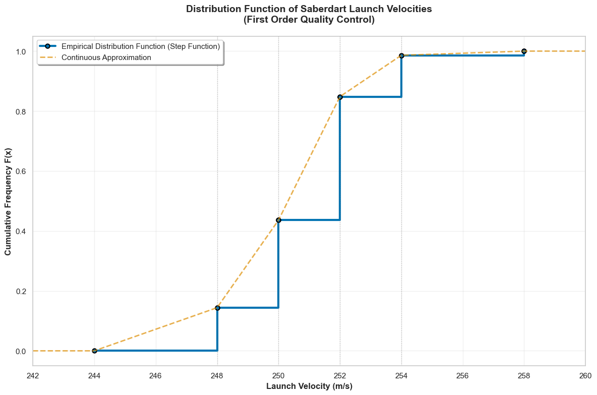
Distribution Law of a Quantitative Variable, Cumulative Distribution Function
The empirical law or distribution of a variable \(X\) over a population \(\Omega\) is defined by the frequency of each class defined by the variable \(X\).
- If \(X\) is qualitative or discrete, its law is defined by the frequency of each subpopulation of the type \(\{X = x_i\} = \{\omega \in \Omega, X(\omega) = x_i\}\).
- If \(X\) is continuous and its possible values are distributed in classes \(C_i\), the empirical law of \(X\) is defined by the frequency of each subpopulation \(\{X \in C_i\} = \{\omega \in \Omega, X(\omega) \in C_i\}\). Examples 4 and 6 illustrate this concept, respectively for a qualitative variable and a continuous variable whose values are grouped into classes
Definition
The empirical distribution function of \(X\) is the function, denoted \(F_{X}\), which associates to each \(x\in \mathbb{R}\) the frequency of the sub-population \(\{X \leq x\}\): \(\begin{aligned} F_{x} : \ &\mathbb{R} \to \mathbb{R} \\ &x \mapsto F_{x}(x) = \frac{\text{Card} \{\omega \in \Omega, X(\omega) \leq x\}}{\text{Card}\Omega} \end{aligned}\) Note this definition always defines \(F_{X}\) on the entire \(\mathbb{R}\), even for values that are not a priori possible values of \(X\) (in which case the sub-population \(\{X \leq x\}\) still makes sense, and is possibly empty).
An empirical distribution function is always increasing on \(\mathbb{R}\), with limits \(0\) at \(-\infty\) and \(1\) at \(+\infty\). Since the population \(\Omega\) is finite, it is actually always a step function. In practice, for a population that can be “assimilated” to an infinite population and a continuous characteristic \(X\), the distribution function \(F_{X}\) is itself assimilated to a continuous increasing function from \(0\) to \(1\).
This figure illustrates this with the data from Example 6. Of course, since we only have partial data, the calculable points of the empirical distribution function are “connected” (interpolated) in a plausible way to effectively give a continuous function.
import matplotlib.pyplot as plt
import numpy as np
import seaborn as sns

sns.set_theme(style="whitegrid")
colorblind_palette = sns.color_palette("colorblind")

# Data from Example 6: Saberdart Launch Velocities
velocity_classes = ['[244;248]', '[248;250]', '[250;252]', '[252;254]', '[254;258]']
class_centers = [246, 249, 251, 253, 256]  # Midpoints of each class
counts = [72, 146, 206, 69, 7]
cumulative_counts = np.cumsum(counts)
total_count = sum(counts)
cumulative_freq = cumulative_counts / total_count

# For the distribution function, we need the upper class boundaries
upper_boundaries = [248, 250, 252, 254, 258]
lower_boundaries = [244, 248, 250, 252, 254]

# Create the step function data for empirical distribution
step_x = [244]  # Start from the minimum
step_y = [0.0]   # Start at 0%

for i, (upper, freq) in enumerate(zip(upper_boundaries, cumulative_freq)):
    step_x.extend([upper, upper])
    step_y.extend([freq, cumulative_freq[i] if i < len(cumulative_freq)-1 else 1.0])

# Also create a smooth interpolation for the "assimilated continuous" version
x_smooth = np.linspace(242, 260, 200)
y_smooth = np.interp(x_smooth, step_x, step_y)

# Create the figure
plt.figure(figsize=(12, 8))

# Plot the empirical step function
plt.step(step_x, step_y, where='post',
         linewidth=3,
         color=colorblind_palette[0],
         label='Empirical Distribution Function (Step Function)',
         marker='o',
         markersize=6,
         markerfacecolor=colorblind_palette[0],
         markeredgecolor='black',
         markeredgewidth=1.5)

# Plot the smooth interpolation
plt.plot(x_smooth, y_smooth,
         linewidth=2,
         color=colorblind_palette[1],
         linestyle='--',
         alpha=0.7,
         label='Continuous Approximation')

# Add class boundaries as vertical lines
for boundary in upper_boundaries[:-1]:  # Don't include the last one
    plt.axvline(x=boundary, color='gray', linestyle=':', alpha=0.5, linewidth=1)

# Customize the plot
plt.title('Distribution Function of Saberdart Launch Velocities\n(First Order Quality Control)',
          fontweight='bold', fontsize=14, pad=20)
plt.xlabel('Launch Velocity (m/s)', fontweight='bold')
plt.ylabel('Cumulative Frequency F(x)', fontweight='bold')
plt.xlim(242, 260)
plt.ylim(-0.05, 1.05)
plt.grid(True, alpha=0.3)

plt.legend(loc='upper left', frameon=True, fancybox=True, shadow=True)
plt.tight_layout()
plt.show()
Common Statistical Measures
Let’s consider a quantitative variable \(X\) for which we have, in the discrete case, \(n\) values denoted as \(x_1, \ldots, x_n\). If \(X\) is continuous, we usually have a discretization of the data into \(k\) classes, which are generally intervals of \(\mathbb{R}\). We denote these classes as \([e_{i-1}, e_i[\).
Calculating characteristic quantities related to the empirical distribution of \(X\) often allows summarizing essential information. We present some of these quantities, distinguishing between position parameters (also sometimes called central tendency parameters) and dispersion parameters.
Position Parameters
Definition: Mean
The mean of the characteristic \(X\) is the quantity \(\bar{x} = \frac{1}{n} \sum_{i=1}^{n} x_i\).
The mean is the most commonly used parameter. Easy to calculate, it has the disadvantage of being very sensitive to the removal or addition of extreme or “aberrant” values. It is said to be a non-robust statistic.
Example 7
The table below presents the statistical series giving the blaster accuracy ratings (on a scale of 0-100) for 11 stormtroopers during training exercises.
| Accuracy Rating | 50 | 40 | 30 | 60 | 70 |
|---|---|---|---|---|---|
| Count | 2 | 2 | 2 | 1 | 4 |
The mean accuracy rating for these stormtroopers is then:
\(\bar{x} = \frac{1}{11}(2\times50 + 2\times40 +2\times30 +1\times60 +4\times70) =\frac{580}{11}\approx 52.73\) The mean accuracy rating is therefore approximately 52.7%.
Proposition: Affine Transformation of the Mean
If an affine transformation of the variable \(X\) is performed, then the mean \(\bar{x}\) undergoes the same affine transformation.
In other words, if \(Y = aX + b\) with \(a, b \in \mathbb{R}\), then:
\[\bar{y} = a\bar{x} + b\]In the case of a continuous variable, we generally assume that the distribution of observations is uniform within each class. Then the average value of the observations in the class \([e_{i-1}, e_i[\) is \(x_i = \frac{1}{2}(e_{i-1} + e_i)\).
In the case where there are \(k\) classes, we can then calculate the mean \(\bar{x}\) as:
\[\bar{x} = \frac{1}{n} \sum_{i=1}^{k} n_i x_i = \sum_{i=1}^{k} f_i x_i\]where \(n_i\) and \(f_i\) denote the count and frequency of the class \([e_{i-1}, e_i[\), respectively.
Definition: mode
The mode, or modal class, of a statistical distribution is the value (or class) of the characteristic that corresponds to the highest frequency.
In Example 7, the mode is 70, corresponding to the most common accuracy rating.
The mean is a non-robust parameter, meaning it is sensitive to aberrant values (too small or too large). To eliminate the role of aberrant values, we define another position parameter: the median. Intuitively, it is a value, denoted as \(M_e\), that divides the statistical distribution into two subpopulations of equal size. More precisely, we have the following definition.
Definition: Median
The median of the characteristic \(X\) is any number \(M_e\) such that the frequency of the subpopulation \(\{X \leq M_e\}\) is greater than or equal to \(\frac{1}{2}\) and the frequency of the subpopulation \(\{X \geq M_e\}\) is also greater than or equal to \(\frac{1}{2}\):
\[f(\{X \leq M_e\}) \geq \frac{1}{2} \quad \text{and} \quad f(\{X \geq M_e\}) \geq \frac{1}{2}\]In practice, after sorting the observations in ascending order, the median is the value of the observation at rank \(\frac{n+1}{2}\) if \(n\) is odd. If \(n\) is even \((n = 2p)\), by convention, we choose the midpoint of the interval \([x_p, x_{p+1}]\).
Let’s take the data from Example 7, and sort them in increasing order, each repeated a number of times equal to its count:
30, 30, 40, 40, 50, 50, 60, 70, 70, 70, 70
We obtain a median \(M_{e}\) equal to 50, i.e., a median accuracy rating of 50%.
Remark
The median is more robust than the mean but its properties make it more difficult to use.
Definition: Quartiles
The quartiles \(Q_1\), \(Q_2\), and \(Q_3\) are, analogously, values that divide the population into four subpopulations of equal size, each representing \(25\%\) of the total population.
There are different methods to obtain quartiles. In the case of a discrete variable, the most common method is to determine the medians of each of the two subpopulations delimited by the median \(M_e\) to obtain the quartiles \(Q_1\) and \(Q_3\).
In the case of example 7, we have \(Q_{1}=40\), which means that at least 25% of the stormtroopers in this unit have an accuracy rating less than or equal to 40%.
Remark
The interquartile range \(\lvert Q_3 - Q_1 \rvert\) is sometimes used to measure the dispersion of data around the median.
Similarly, given an integer \(p \geq 2\), we can define quantiles, which are values of the characteristic that divide the population into \(p\) subpopulations of equal size. For example, the deciles of a statistical series divide the series into ten equal parts. In practice, only the first and last deciles, denoted as \(D_1\) and \(D_9\), are used.
Remark
In the case of a continuous variable, we can use the empirical cumulative distribution function \(F_X\) to determine the quantiles. For example, if the function \(F\) is continuous and strictly increasing, then it establishes a bijection from \(\mathbb{R}\) to \(]0, 1[\), and we have:
\[Q_1 = F_X^{-1}(0.25) \quad M_e = F_X^{-1}(0.5) \quad Q_3 = F_X^{-1}(0.75)\]In practice, we obtain approximate values of these quantities by performing linear interpolation.
Once the quartiles and deciles have been calculated, we can represent the data synthetically using a box plot (also known as a box-and-whisker plot). The central part of the box is a rectangle whose length is the interquartile range \(\lvert Q_3 - Q_1 \rvert\). The “whiskers” are segments that extend on either side of the box to the first decile \(D_1\) for the lower whisker and to the last decile \(D_9\) for the upper whisker. These whiskers are said to be trimmed. Less common are untrimmed whiskers, which extend to the minimum and maximum of the distribution (which may be aberrant values).
There is also a variant of this representation called a Tukey diagram, in which the length of the whiskers is fixed at 1.5 times the interquartile range. This results in symmetric whiskers, which may not correspond to the actual empirical distribution.
The advantage of box plots is that they allow easy (visual) comparison of several data series.
Dispersion Parameters
Position characteristics are generally not sufficient to summarize data. To complement them, we calculate dispersion parameters that account for the more or less pronounced “spread” of observed values.
Definition: spead
The range (or spread) is the difference between the extreme values of the characteristic:
\[w = x_{\max} - x_{\min}\]The range is a coarse parameter, non-robust in that its sensitivity to aberrant values is extreme.
Definition: Variance
The variance of the variable \(X\) is the quantity:
\[\sigma^2 = \frac{1}{n} \sum_{i=1}^{n} (x_i - \bar{x})^2\]which represents the mean of the squares of the deviations between the observations and their mean.
The standard deviation of \(X\) is the square root \(\sigma\) of the variance.
The variance of \(X\) can also be denoted as \(\mathbb{V}(X)\), but we will tend to use this notation only in the context of random variables.
The variance plays a fundamental role in statistics due to its properties (which other dispersion parameters do not have). In practice, it is often calculated using the following relationship, which is demonstrated by expanding the formula.
Proposition: Usual Formula for Calculating Variance
\[\sigma^2 = \frac{1}{n} \sum_{i=1}^{n} x_i^2 - \bar{x}^2\](mean of squares minus square of the mean).
One of the important properties of variance concerns the effect of an affine transformation (the effect of such an affine transformation on the mean was mentioned in Proposition 1).
Proposition: Effect of an Affine Transformation on Variance
If an affine transformation of the data is performed, then the variance is multiplied by the square of the slope of the transformation.
In other words, if we set \(Y = aX + b\) with \(a, b \in \mathbb{R}\), then:
\[\sigma_Y^2 = a^2 \sigma_X^2\]Let’s take the data from Example 7. We saw that \(\bar{x} \approx 52.73\). We therefore have: \(\sigma^{2}=\frac{1}{11}[ 2 \times 50^{2}+2\times40^{2}+2\times30^{2}+1\times60^{2}+4\times70^{2}] - 52.73^{2}\approx 237.7\) hence the standard deviation \(\sigma \approx 15.42\). This standard deviation is a measure of dispersion around the mean value.
As a final common dispersion parameter, we mention the interquartile range, already encountered:
\[I_Q = |Q_3 - Q_1|\]Distributions with two variables
Let’s now study a population of size \(n\) according to two variables \(X\) and \(Y\), which can be qualitative or quantitative,without necessarily being of the same nature.
Example 9:
We recorded the height (in cm) and midi-chlorian count of a population consisting of 200 Jedi Padawans from the Coruscant Jedi Temple.
Example 10
In a survey of Time Lord academy graduates, we recorded for each TARDIS the primary console room theme (Classic, Coral, Victorian, Crystal, Steam-punk) and the average travel accuracy percentage.
If \(X{\Omega}\) is finite, its \(r\) modalities are denotes \(x_{1}, x_{2}, \ldots, x_{i}, \ldots x_{r}\). If its values are distributed into classes, these are denoted \(C_{1}, C_{2}, \ldots, C_{i}, \ldots, C_{r}\).
Similarly, if \(Y(\Omega)\) is finite, we denote \(y_{1}, \ldots, y_{j}, \ldots ,y_{s}\) its elements. If the values of \(Y\) are distributed into classes, these are denotes \(D_{1},\ldots, D_{j}, \ldots, D_{s}\).
The distribution of the \(n\) observations of these variables on the population \(\Omega\) according to the modalities or classes of \(X\) and \(Y\) is presented in the form of a double entry table, called a contingency table:
| \(X\)\ \(Y\) | \(D_1\) | \(\ldots\) | \(D_j\) | \(\ldots\) | \(D_s\) | Total |
|---|---|---|---|---|---|---|
| \(C_1\) | \(n_{11}\) | \(\ldots\) | \(n_{1j}\) | \(\ldots\) | \(n_{1s}\) | n_{1.} |
| \(\vdots\) | \(\vdots\) | \(\vdots\) | \(\vdots\) | \(\vdots\) | ||
| \(C_i\) | \(n_i1\) | \(\ldots\) | \(n_ij\) | \(\ldots\) | \(n_is\) | \(n_i.\) |
| \(\vdots\) | \(\vdots\) | \(\vdots\) | \(\vdots\) | \(\vdots\) | ||
| \(C_r\) | \(n_{r1}\) | \(\ldots\) | \(n_{rj}\) | \(\ldots\) | \(n_{rs}\) | \(n_{r.}\) |
| Total | \(n_{.1}\) | \(\ldots\) | \(n_{.j}\) | \(\ldots\) | \(n_{.s}\) | \(n\) |
In this table, \(n_{ij}\) denote the number of individuals whose observed feature \(X\) belongs to class \(C_{i}\) and whose observed feature \(Y\) belongs to class \(D_{j}\). We therefore write:
\(n_{ij} = \text{Card}(C_{i}\cap D_{j}) \quad \text{and} \quad f_{ij}= \frac{n_{ij}}{n}\) Then \(f_{ij}\) is the frequency of \(C_{i}\cap D_{j}\)
Definition: Joint distribution
The joint distribution of the pair \((X, Y)\) is the data, for each value of \(i\) and \(j\), of the frequency \(f_{ij}\).
We also define:
- The marginal count and marginal frequency of \(X\) for class \(C_i\):
- The marginal count and marginal frequency of \(Y\) for class \(D_j\):
Definition: Conditional distribution
The conditional distribution of \(Y\) given \(X \in C_i\) is the data, for all \(j \in \{1, \ldots, s\}\), of the relative frequencies of the classes \(D_j\) with respect to \(C_i\):
\[f_{j/i} = \frac{n_{ij}}{n_{i.}} = \frac{f_{ij}}{f_{i.}}\]The two variables \(X\) and \(Y\) are said to be independent if the conditional distribution of \(Y\) given \(X \in C_i\) does not depend on \(i\).
In the case where \(X\) and \(Y\) are independent, we have:
\[f_{j/i} = \frac{f_{ij}}{f_{i.}} = f_{.j} \quad \text{or equivalently} \quad f_{ij} = f_{i.} \times f_{.j}\]All these definitions will be found in the part dedicated to probabilities and random variables.
Example 11
In a group of 100 Starfleet officers from different postings, some were assigned to Constitution-class starships (like the Enterprise) and others to smaller vessels like Oberth-class science ships. All officers underwent the same command training. After one year, each officer was evaluated on their mission success rate. The table below gives the distribution of results.
| High success rate | Moderate success rate | Low success rate | |
|---|---|---|---|
| Constitution-class | 36 | 12 | 2 |
| Oberth-claqs | 18 | 20 | 12 |
The marginal distributions of the variables \(X\), which indicates whether an officer serves on a Constitution-class or Oberth-class vessel, and \(Y\), which indicates the mission success rate category, are given by the following tables:
| \(x_i\) | Constitution-class | Oberth-class |
|---|---|---|
| \(f_{i.}\) | 50% | 50% |
| \(y_j\) | High | Moderate | Low |
|---|---|---|---|
| \(f_{.j}\) | 54% | 32% | 14% |
The conditional distribution of \(Y\) given that an officer serves on a Constitution-class vessel is given by the following table:
| \(y_j\) given \(X\) = Constitution | High | Moderate | Low |
|---|---|---|---|
| \(f_{j\lvert1}\) | \(\frac{36}{50}=72\%\) | \(\frac{12}{50}=54\%\) | \(\frac{2}{50}=4\%\) |
Similarly, the conditional distribution of \(Y\) given that an officer serves on an Oberth-class vessel is given by:
| \(y_j\) given \(X\) = Oberth | High | Moderate | Low |
|---|---|---|---|
| \(f_{j\lvert2}\) | \(\frac{18}{50}=36\%\) | \(\frac{20}{50}=40\%\) | \(\frac{12}{50}=24\%\) |
By comparing the conditional distributions \(f_{j\lvert1}\) and \(f_{j\lvert2}\), we are tempted to assert that the variables \(X\) and \(Y\) are not independent and conclude that vessel class affects mission success rates. However, we must be cautious because the studied population is a sample of a larger population, that of all Starfleet officers. The statistical proof of the effect of vessel class on success rates will then involve a statistical test of independence of \(X\) and \(Y\) that takes into account statistical randomness.